Equivariance Properties in Machine Learning
Introduction
When we think about the signs for what is a good model, we first look to notions of accuracy, precision, recall and the like. Evaluating these metrics typically require a ground truth to evaluate against, and is rarely the case that a machine learning practitioner will not have at least a few examples to test on.
In medical imaging deep learning is applied to make measurements about our bodies such as organ size, which helps us gain understand our health. In order for any measurement to be useful, it should be invariant to small changes like the position of the patient, while sensitive to physiological changes such as the progression of a disease.
This sameness property is also desired in machine learning, the idea that if we make changes to a model input, the output of the model should change in a predictable manner (or not change). One example is taking a cat picture and flipping it vertically should cause a good classification model to still predict a cat class (invariance). And for a segmentation model the mask of the flipped cat should just be the flipped version of the mask predicted on the unflipped image (equivariance).

Data augmentation is the go-to method for making models robust to these kinds of changes and is an implicit way of achieving this by exposing these types of scenarios (rotations, brightness changes, noise) to the model during the training process.

We are often quick to instinctively apply data augmentation, and are happy with the outcome so long is the performance improves on our validation set. It is rarer that we verify if in doing so did the models actually learn to be robust to this kind of noise. I will take a step further by picking an individual image and observe how robust the prediction of the model is to varying levels of data augmentation.
Dataset
- I will be using the Leeds Butterfly Dataset consisting of 832 images in total of 10 types of butterflies.

- The masks are binary and do not take into account the type of butterfly, so the task is foreground segmentation of the butterfly
- We resize the images to
(256, 256)when training the models, and pad to (384, 384) with black pixels to perform rotations of the mask later on without losing information at the corners of the mask - The values are normalised with mean
(0.485, 0.456, 0.406)and standard deviation(0.229, 0.224, 0.225) - 20% of the images will be reserved for validation
Models
4 models will be trained in total using 2 sets of data augmentation pipelines and 2 model architectures. These a regular U-Net with Group Normalisation layers with a sigmoid activation layer is applied to the logits to get the foreground probability as there is only one foreground class.
The second model is a U-Net where the Convolutions are replaced with Group Convolutions that run on group feature maps. More details can be found at the University of Amsterdam’s GDL tutorials describing Group Theory in Machine Learning, and there is also the original Cohen/Welling paper on Group Equivariant Convolutional Networks. We use the cyclic rotation group of order 4 corresponding to 90 degree rotations. This allows the model to be robust to rotation without having to perform data augmentation.

Model Parameters
- U-Net configurations for both the original and Group U-Net use 4 downsampling blocks with residual connections from the input of the block to its output.
- As the the group convolutions operate on the group features the number of trainable parameters is higher. We halve the number of filters in each of the group convolution layers which brings the number of trainable parameters to around the same.
- U-Net -
[32, 32, 64, 64]filters in the downsampling blocks and the reverse during upsampling - Group U-Net -
[16, 16, 32, 32]filters in the downsampling blocks and the reverse during upsampling
- U-Net -
- In all networks we perform Group Normalisation on the channels
Augmentation Sets
We create a base set of data augmentation using Albumentations which includes just the preprocessing steps such as normalisation, and constant padding around the borders.
Each model type was additionally trained using a fuller set of augmentations such as rotations of up to 90 degrees, brightness/contrast changes, and color adjustments.
import albumentations as A

from albumentations.pytorch.transforms import ToTensorV2
from albumentations.augmentations.geometric.rotate import SafeRotate
from albumentations.augmentations.transforms import ColorJitter
from albumentations.augmentations.transforms import RandomBrightnessContrast


preprocessing = A.Compose([
	A.PadIfNeeded(width, width, border_mode=cv2.BORDER_CONSTANT, value=0),
	A.Normalize(),
	ToTensorV2(),
])

full_transform = A.Compose([
	ColorJitter(),
	RandomBrightnessContrast(),
	SafeRotate(limit=90),
	preprocessing,
])
Training & Evaluation
- We train each of the models for 150 epochs
- The
AdamWoptimiser is used with an initial learning rate of 1e-3 and a default weight decay of 1e-2 - A batch size of 16 is used during training
- For loss we use the
BCEWithLogitsLoss - For accuracy we calculate the Intersection over Union (IoU)
- More implementation details for this experiment can be found here
We monitor the training/validation performance over time and look at the final values. The validation dataset undergoes the base preprocessing but with an additional random number of 90 degree rotations to evaluate the robustness of these models to this particular transformation.
import albumentations as A

val_transform = A.Compose([
	A.RandomRotate90(),
	preprocessing,
])
In addition, we sample a single image and run an additional test:
- Create a set of images consisting of a varying number of rotations from 0 to 360 degrees
- Run the stack through the model
- Invert the masks back to the original orientation of the base image by rotating the mask by the angle in the opposite direction
- Apply centre crop to remove the black borders introduced during preprocessing
- Calculate the intersection over union between the set of predictions and the single unaltered ground truth, and plot these scores as a function of the rotation angle
import cv2
import numpy as np
import torch.nn as nn
import albumentations as A

from albumentations.pytorch.transforms import ToTensorV2
from torchvision.transforms.functional import rotate


def batched_prediction(
    model: nn.Module,
    image: np.ndarray,
    angles: List[float],
    pad_size: int = 384,
) -> torch.Tensor:
    image = cv2.cvtColor(image, cv2.COLOR_BGR2RGB)
    h, w, _ = image.shape

    # Pad and rotate images
    preprocessing = A.Compose([
        A.PadIfNeeded(pad_size, pad_size, border_mode=cv2.BORDER_CONSTANT, value=0),
        A.Normalize(),
        ToTensorV2(),
    ])
    image = preprocessing(image=image)["image"]
    images = torch.stack([rotate(image, angle) for angle in angles])

    batch_size = 4
    predictions = []
    for i in range(0, images.shape[0], batch_size):
        pred = torch.sigmoid(model(images[i:i+batch_size])) > 0.5
        pred = torch.squeeze(pred)
        predictions.append(pred)

    # Invert padding and centre crop
    predictions = torch.concat(predictions, dim=0)
    predictions = torch.concat([
        rotate(repeat(pred, "... -> 1 ..."), -angle) for pred, angle in zip(predictions, angles)
    ], dim=0)
    crop_w = (pad_size - w) // 2
    crop_h = (pad_size - h) // 2
    predictions = predictions[:, crop_h:-crop_h, crop_w:-crop_w]
    return predictions
Results
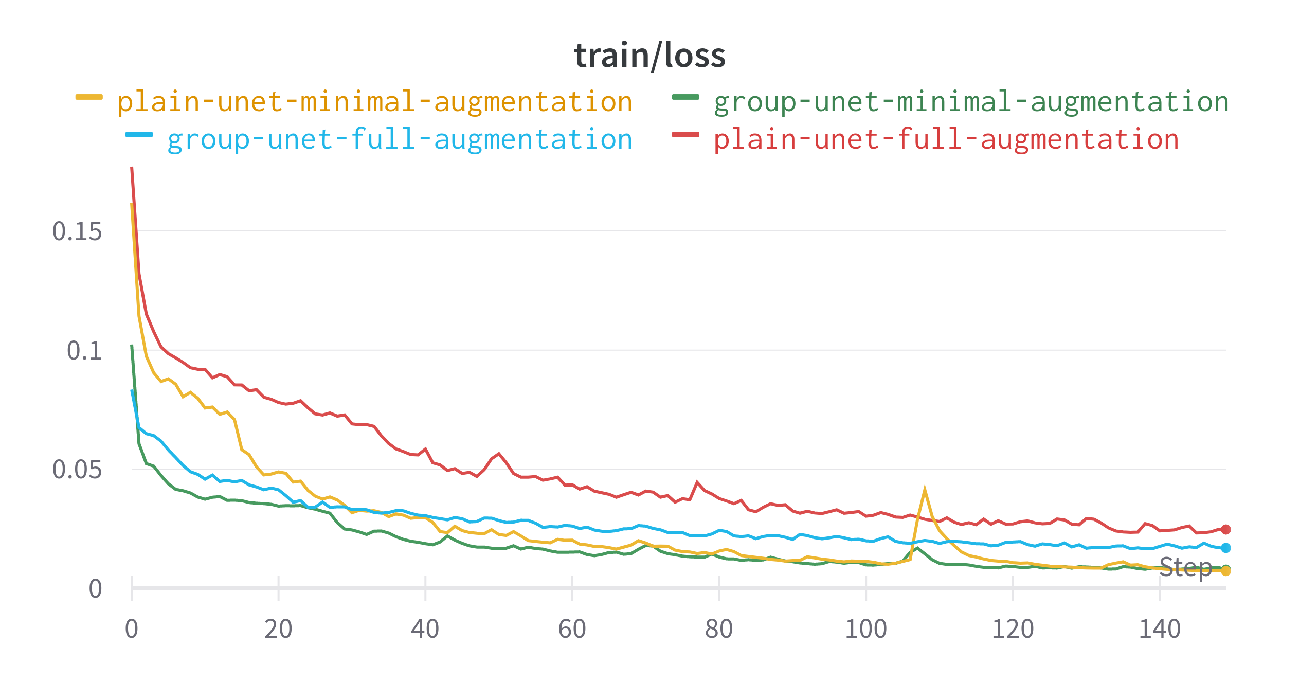
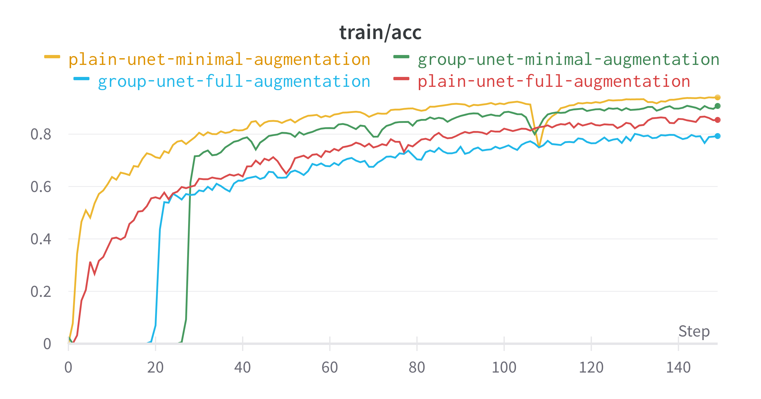
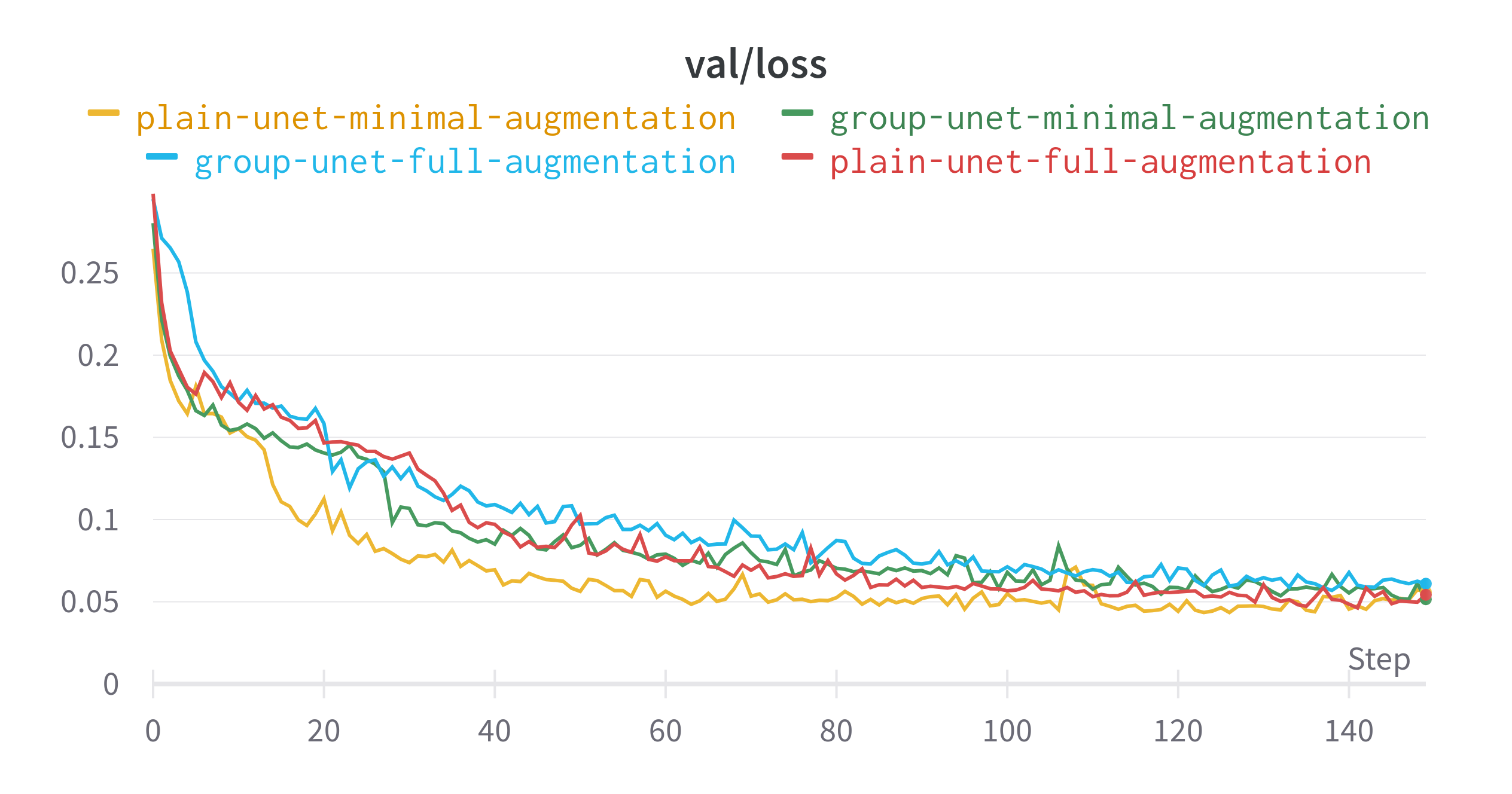
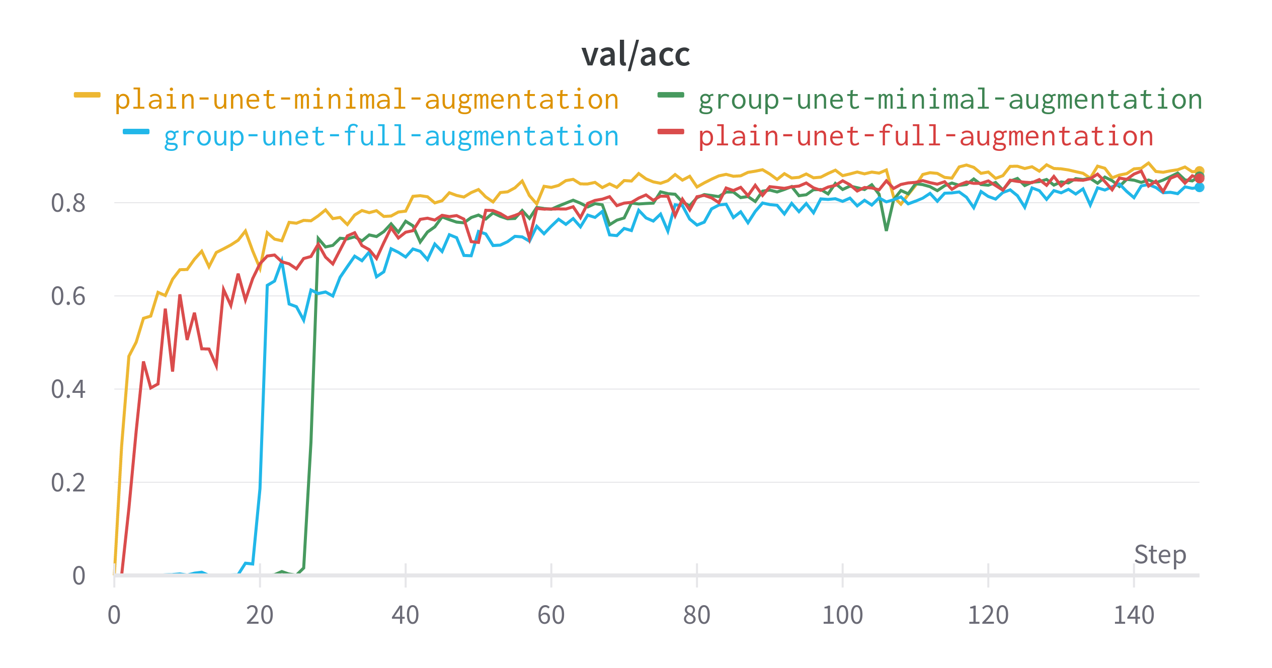
The plain U-Net with little augmentation did best in terms of learning the data distribution that it was presented. Despite having less augmentation and no specialised layers, this model had the highest validation dice score. The difference between the best and worst performing model for this metric is around 0.03. The gap in validation loss is even smaller.
- The original U-Net with minimal preprocessing performed the best in terms of learning its data distribution
- Many of the Group U-Nets did not predict anything for several epochs
- The two models trained with just the base preprocessing saw a drop in performance around epoch 110
- Using the full set of augmentations resulted in models that performed less than their minimal counterparts.
Final Epoch Performance
| Model | Data Augmentation | Train IoU | Train Loss | Validation IoU | Validation Loss |
|---|---|---|---|---|---|
| Plain U-Net | Minimal | 0.9404 | 0.007263 | 0.8678 | 0.05585 |
| Plain U-Net | Full | 0.8543 | 0.0247 | 0.8522 | 0.05425 |
| Group U-Net | Minimal | 0.9076 | 0.007864 | 0.8563 | 0.05154 |
| Group U-Net | Full | 0.7927 | 0.01696 | 0.8332 | 0.06099 |


Rotated Predictions
For each of the models we predict on a single image rotated with multiple angles and plot the dice scores for each angle. In this example we see that despite not having the highest IoU, the Group U-Net predictions are more consistent with the angle. Whereas for other models the IoU score can change as much as 0.04 depending on the chosen angle.
In the Group U-Net Full Augmentation and Plain U-Net minimal augmentation setups it is easy to see that there is a lot of variance with predicting the main body of the butterfly.
Occasionally the models will segment the border of the image as a butterfly, but I think this is due to my choice of zero padding and the model associating dark pixels with the wings of the butterfly as is the case for a few of the species in this dataset.
Plain U-Net Full Augmentation

Plain U-Net Minimal Augmentation

Group U-Net Full Augmentation

Group U-Net Minimal Augmentation

Conclusion
The models trained here have a lot of room for improvement. The key message is that thinking beyond comparisons to a ground truth like equivariance properties can be a useful test in situations where labels are scarce or even impossible to obtain.
Regardless of how you design your model, one can test explicitly test equivariance by taking an inputs and perturbing it by a range of values, and observing what happens. If your predictions are consistent across a range of perturbations, then that might be one sign of a good model.